GAMES101-现代计算机图形学笔记

好的画面：技术层面-看画面够不够亮（全局光照）

课程主题：

光栅化
曲线和曲面/几何
光线追踪
动画/模拟

光栅化：把三维空间的几何形体显示在屏幕上的过程就叫光栅化。

几何：如何在图形中表达曲面/曲线。

光线追踪：从相机中反向发射光线模拟现实的光照，

动画/模拟：模拟动画的帧、或者质点弹簧系统

图形学依赖：

基础数学
- 线性代数
- 微积分
- 统计
基础物理
- 光学
- 力学
其他
- 信号处理
- 数值分析
美学

线性代数

向量

在图形学中，我们默认方向就是一个单位向量，即：
$$
\hat{a} = \frac{\vec{a}}{\vert\vert\vec{a}\vert\vert}
$$

a_hat也就是单位向量是由一个向量除以它的长度得到的。

在图形学中，默认一个向量是列向量，即：

$$
A = \left(
\begin{matrix}
x \
y \
\end{matrix}
\right)
$$

A的转置即行向量：
$$
A^T = \left(
\begin{matrix}
x ,& y \
\end{matrix}
\right)
$$
可以得到：
$$
\vert\vert A \vert\vert = \sqrt{x^2 + y^2}
$$

向量乘法

点乘

向量点乘最后得到的还是一个数，即以下公式：

$$
\vec a \cdot \vec b = \vert\vert {\vec {a}} \vert\vert \ \vert\vert {\vec {b}}\vert\vert \ cos\theta
$$

我们可以由此来计算两个向量之间的夹角cosθ
$$
cos\theta = \frac{\vec a \cdot \vec b}{\vert\vert {\vec {a}} \vert\vert \ \vert\vert {\vec {b}}\vert\vert}
$$
特别是用来计算单位向量的夹角：
$$
cos\theta = {\hat {a}} \cdot {\hat {b}}
$$
同时，点乘满足以下规律：

交换律
结合律
分配律

在笛卡尔直角坐标系下，向量的点乘可以写成：

二维

$$
\vec a \cdot \vec b = \left(
\begin{matrix}
x_a \
y_a \
\end{matrix}
\right)

      \cdot
      
      \left(
     \begin{matrix}
       x_b  \\
       y_b  \\
      \end{matrix}
      \right)
      
      = x_a x_b + y_a y_b

三维

$$
\vec a \cdot \vec b = \left(
\begin{matrix}
x_a \
y_a \
z_a
\end{matrix}
\right)

      \cdot
      
      \left(
     \begin{matrix}
       x_b  \\
       y_b  \\
       z_b
      \end{matrix}
      \right)
      
      = x_a x_b + y_a y_b + z_a z_b

在图形学中，点乘主要用来：

找到两个向量之间的夹角
找到一个向量投影到另一个向量是什么样的

图形学中投影的用处：

测量两个向量有多么的接近
将一个向量分解成两个向量
确定向量是向前还是向后

可以从以下式子得出两个向量的方向：
$$
\vec a \cdot \vec b > 0 ，\vec a \cdot \vec c < 0
$$

叉乘

两个向量的叉乘仍然是一个向量：

两个向量的叉乘的结果与这两个向量都垂直。
叉乘的结果通过右手（螺旋）定律判断方向
可以建立一个三维空间的直角坐标系

上面的规则可以用一个公式来表示：
$$
\vec x \times \vec y = + \vec z
$$

叉乘在笛卡尔直角坐标系中可以表示为：
$$
\vec a \times \vec b = \left(
\begin{matrix}
y_a z_b - y_b z_a \
z_a x_b - x_a z_b \
x_a y_b - y_a x_b
\end{matrix}
\right)
$$

$$
\vec a \times \vec b = A *b = \left(
\begin{matrix}
0 & -z_a &y_a \
z_a & 0 & -x_a \
-y_a & x_a & 0
\end{matrix}
\right)

                              \left(
                             \begin{matrix}
                               x_b  \\
                               y_b  \\
                               z_b
                              \end{matrix}
                              \right)

叉乘在图形学的作用：

判定左/右
判断内/外

如果：
$$
\vec a \times \vec b > 0
$$
那么，a在b的左侧

如果：
$$
\overrightarrow{AB} \times \overrightarrow{AP} > 0 ,\ \overrightarrow{BC} \times \overrightarrow{BP} > 0,\ \overrightarrow{CA} \times \overrightarrow{CP} > 0
$$
那么P点在三角形的内部。

不过顺时针还是逆时针，如果P点一定在三条边的左边或者一定在三条边的右边，那么P点在三角形的内部。

将P向量分解到uvw坐标系中，相当于
$$
\vec p = k_u \vec u + k_v \vec v + k_w \vec w
$$
这是因为uvw都是单位向量，他们的点乘就是p的长度乘以cosθ，也就是在每个方向上的分量k。

矩阵

矩阵是一堆mxn数字的数组，其中m表示行，n表示列
逐元素加法和标量乘法

矩阵的乘法

满足：

(MxN) (NxP) = (MxP)
元素（i，j）的值是由A矩阵的i行和B矩阵的j列的点积得到的。

性质：

没有任何的交换律
结合律和分配律
- AB(C) = A(BC)
- A(B+C) = AB + AC
- (A+B)C = AC + BC

矩阵的转置的特殊性质:
$$
(AB)^T = B^TA^T
$$

单位矩阵：
$$
AA^{-1} = A^{-1}A = I
$$

$$
(AB)^{-1} = B^{-1}A^{-1}
$$

向量的乘积可以写成矩阵的形式：

变换 - Transformation

线性变换

线性变换包括缩放（Scale）、剪切（Shear）、旋转（Rotate）

旋转操作默认是绕原点，逆时针旋转。在旋转矩阵中，它的逆等于它的转置，即这是一个正交矩阵。

齐次坐标

平移操作不是线性变换，但我们不希望平移变换被当成特殊的变换，有没有办法把所有的变换使用一种变换表示？

引入齐次坐标！

向量具有平移不变性。

观测变换 - Viewing transformation

观测变换包含以下变换：

View(视图) / Camera transformation
Proiection(投影) transformation
- Orthographic(正交) projection
- Persoective(透视) projection

MVP矩阵：Model transformation、View transformation、Projection transformation

视图变换 - View / Camera transformation

投影变换 - Proiection transformation

透视投影可以表示为以下的形式：
$$
M_{persp} = M_{ortho}M_{persp \to ortho}
$$

它首先经过一个压缩的操作然后再进行正交变换。

正交投影：

$$
tan(\frac{FOV}{2}) = \frac{t}{\vert n \vert} \tag{1}
$$

$$
Right = Top * Aspect \tag{2}
$$

M_ortho
$$
\left[
\begin{matrix}
\frac{1}{AspectT op} & 0 & 0 &0 \
0 & \frac{1}{top} & 0 &0\
0 & 0 & -\frac{2}{Far - Near} &-\frac{Far + Near}{Far - Near}\
0 & 0 & 0 &1
\end{matrix}
\right] \tag{3}
$$
M_persp2ortho
$$
\left[
\begin{matrix}
Near & 0 & 0 &0 \
0 & Near & 0 &0\
0 & 0 & Far + Near &- FarNear\
0 & 0 & 1 &0
\end{matrix}
\right] \tag{4}
$$
M_projection
$$
\left[
\begin{matrix}
\frac{cot(\frac{FOV}{2})}{Aspect} & 0 & 0 &0 \
0 & cot(\frac{FOV}{2}) & 0 &0\
0 & 0 & -\frac{Far + Near}{Far - Near} &-\frac{2 Far*Near}{Far - Near}\
0 & 0 & -1 &0
\end{matrix}
\right] \tag{5}
$$

M_projection = M_ortho * M_persp2ortho

视口变换

在MVP变换之后，会使用视口变换将[-1,1]^3这个空间映射到屏幕空间中去。

[-1,1]^3是由投影矩阵将空间拉伸而成的空间，默认中心原点是摄像机所在的点。

$$
\left[
\begin{matrix}
\frac{width}{2} &0 &0 &\frac{width}{2} \
0 &\frac{height}{2} &0 &\frac{height}{2}\
0 &0 &0 &0\
0 &0 &0 &0
\end{matrix}
\right]
$$

作业1

模型矩阵：

Eigen::Matrix4f get_model_matrix(float rotation_angle)
{
    Eigen::Matrix4f model = Eigen::Matrix4f::Identity();

    // TODO: Implement this function
    // Create the model matrix for rotating the triangle around the Z axis.
    // Then return it.

    float rotation_radians = rotation_angle * MY_PI / 180.0;
    float cos_value = cos(rotation_radians);
    float sin_value = sin(rotation_radians);

    model << 
        cos_value, -sin_value, 0, 0, 
        sin_value, cos_value, 0, 0, 
        0, 0, 1, 0, 
        0, 0, 0, 1;

    return model;
}

修改之后的投影矩阵：

Eigen::Matrix4f get_projection_matrix(float eye_fov, float aspect_ratio, float zNear, float zFar)
{

    Eigen::Matrix4f projection = Eigen::Matrix4f::Identity();
    
    float fov = eye_fov * MY_PI / 180.0f;
    // zNear is negative, need * -1.
    float top = -zNear * tan(fov * 0.5);
    Eigen::Matrix4f M_ortho;
    Eigen::Matrix4f M_persp2ortho;

    M_ortho <<
        1 / (aspect_ratio * top), 0, 0, 0,
        0, 1 / top, 0, 0,
        0, 0, -2 / zFar - zNear, -(zFar + zNear) / (zFar - zNear),
        0, 0, 0, 1;

    M_persp2ortho <<
        zNear, 0, 0, 0,
        0, zNear, 0, 0,
        0, 0, zNear + zFar, -zNear * zFar,
        0, 0, 1, 0;

    projection = M_ortho * M_persp2ortho;

    return projection;
}

旋转矩阵：

Eigen::Matrix4f get_rotation(Eigen::Vector3f axis, float angle)
{
    Eigen::Matrix4f model = Eigen::Matrix4f::Identity();

    float rotation_radians = angle * MY_PI / 180.0;
    float cos_value = cos(rotation_radians);
    float sin_value = sin(rotation_radians);

    Eigen::Matrix4f I = Eigen::Matrix4f::Identity();

    Eigen::Matrix4f M_axis;
    M_axis << axis.x(), axis.y(), axis.z(), 0;
    Eigen::MatrixXf M_axis_transposed = M_axis.transpose();

    Eigen::Matrix4f N;
    N << 0, -M_axis.z(), M_axis.y(), 0,
        M_axis.z(), 0, -M_axis.x(), 0,
        -M_axis.y(), M_axis.x(), 0, 0,
        0, 0, 0, 1;

    model = cos_value * I + (1 - cos_value) * M_axis * M_axis_transposed + sin_value * N;

    return model;
}

光栅化 - Rasterization

从零开始写一个光栅化器：https://github.com/ssloy/tinyrenderer/wiki

三角形的离散化

采样：将一个函数离散化的过程

通过判断像素中心点是否在三角形内部来决定是否剔除这个三角形，从而进行采样。

由于采样带来的Artifacs - “Aliasing”

锯齿 - 空间采样
摩尔纹 - 欠采样图片
车轮效应 - 时间采样

走样的本质：

信号（函数）改变太快了，但是采样太慢了。

抗锯齿的实现：

在采样之前先模糊（滤波）

滤波：去掉某些特定的频段

为什么采样速度跟不上信号速度会导致走样？

为什么先滤波在采样能够抗锯齿？

频域

傅里叶展开

频域上的乘积等于时域上的卷积

采样是再重复原始信号的频谱
走样是在采样的过程中由于采样速度小于信号{函数、波}的速度，导致采样点稀疏，进而使得重复的频谱混合，就会发生走样。

反走样

增加采样率（分辨率）
反走样（先模糊再采样）

抗锯齿

Antialiasing By Supersampling

MSAA

没有提高分辨率，而是提高采样点的密度，得到近似三角形的覆盖。

近年的抗锯齿

抗锯齿的开销：

增大了计算量

其他抗锯齿方法

FXAA（Fast Approximate AA）快速近似抗锯齿 - 图像后期处理层面，和采样无关。
TAA （Temporal AA）- 今年兴起，在时间层面的操作。通过复用上一帧，找到临近点。

超分辨率

接近样本不足
从低分辨率到高分辨率
仍然没有解决没有足够样本的问题
DLSS

深度检测

可见性的解决方法：深度缓冲 Z-buffering

为了解决画家算法无法绘制互相遮挡的三角面的缺陷，提出了 Z-buffer。

生成两张图

帧缓存frame buffer存储颜色信息
深度缓冲depth buffer存储深度信息

为了方便计算，z总是正的，z越小越近。

广泛应用在硬件中。

作业2

目标

正确实现三角形栅格化算法。
正确测试点是否在三角形内。
正确实现 z-buffer 算法, 将三角形按顺序画在屏幕上。
用 super-sampling 处理 Anti-aliasing （MSAA）

判断是否在三角形内

static bool insideTriangle(float x, float y, const Vector3f* _v)
{   
    // TODO : Implement this function to check if the point (x, y) is inside the triangle represented by _v[0], _v[1], _v[2]

    float checkPoint_x = x;
    float checkPoint_y = y;

    Eigen::Vector2f AB = Eigen::Vector2f(_v[1].x() - _v[0].x(), _v[1].y() - _v[0].y());
    Eigen::Vector2f BC = Eigen::Vector2f(_v[2].x() - _v[1].x(), _v[2].y() - _v[1].y());
    Eigen::Vector2f CA = Eigen::Vector2f(_v[0].x() - _v[2].x(), _v[0].y() - _v[2].y());
    Eigen::Vector2f AP = Eigen::Vector2f(checkPoint_x - _v[0].x(), checkPoint_y - _v[0].y());
    Eigen::Vector2f BP = Eigen::Vector2f(checkPoint_x - _v[1].x(), checkPoint_y - _v[1].y());
    Eigen::Vector2f CP = Eigen::Vector2f(checkPoint_x - _v[2].x(), checkPoint_y - _v[2].y());

    float cross_AB_AP = AB.x() * AP.y() - AB.y() * AP.x();
    float cross_BC_BP = BC.x() * BP.y() - BC.y() * BP.x();
    float cross_CA_CP = CA.x() * CP.y() - CA.y() * CP.x();

    if (cross_AB_AP > 0 && cross_BC_BP > 0 && cross_CA_CP > 0 ||
        cross_AB_AP < 0 && cross_BC_BP < 0 && cross_CA_CP < 0)
    {
        return true;
    }
    else
    {
        return false;
    }
}

光栅化三角形

void rst::rasterizer::rasterize_triangle(const Triangle& t) {
auto v = t.toVector4();

// TODO : Find out the bounding box of current triangle.
// iterate through the pixel and find if the current pixel is inside the triangle

// If so, use the following code to get the interpolated z value.
//auto[alpha, beta, gamma] = computeBarycentric2D(x, y, t.v);
//float w_reciprocal = 1.0/(alpha / v[0].w() + beta / v[1].w() + gamma / v[2].w());
//float z_interpolated = alpha * v[0].z() / v[0].w() + beta * v[1].z() / v[1].w() + gamma * v[2].z() / v[2].w();
//z_interpolated *= w_reciprocal;

// TODO : set the current pixel (use the set_pixel function) to the color of the triangle (use getColor function) if it should be painted.


//bounding box的实现
float x_max = v[0].x(), x_min = v[0].x(), y_max = v[0].y(), y_min = v[0].y();

for (auto i : v)
{
    if (i[0] < x_min) 
        x_min = i[0];
    if (i[0] > x_max) 
        x_max = i[0];
    if (i[1] < y_min) 
        y_min = i[1];
    if (i[1] > y_max) 
        y_max = i[1];
}

//以下是未进行抗锯齿处理的版本
for (int x = x_min; x < x_max; x++)
{
    for (int y = y_min; y < y_max; y++)
    {
        bool isInsideTriangle = insideTriangle(x, y, t.v);
        if (isInsideTriangle)
        {
            auto result = computeBarycentric2D(x + 0.5, y + 0.5, t.v);
            float alpha, beta, gamma;
            std::tie(alpha, beta, gamma) = result;
            float w_reciprocal = 1.0 / (alpha / v[0].w() + beta / v[1].w() + gamma / v[2].w());
            float z_interpolated = alpha * v[0].z() / v[0].w() + beta * v[1].z() / v[1].w() + gamma * v[2].z() / v[2].w();
            z_interpolated *= w_reciprocal;

            if (z_interpolated < depth_buf[get_index(x, y)])
            {
                Eigen::Vector3f point = Eigen::Vector3f(x, y, z_interpolated);
                set_pixel(point, t.getColor());
                depth_buf[get_index(x, y)] = z_interpolated;
            }
        }
    }
}

实现MSAA的代码：

首先，需要在rasterizer.cpp中，添加深度缓存和颜色缓存：

1 2	std::vector<Eigen::Vector3f> sampleList_frame_buf; std::vector<float> sampleList_depth_buf;

同时需要对他们进行初始化：

void rst::rasterizer::clear(rst::Buffers buff)
{
    if ((buff & rst::Buffers::Color) == rst::Buffers::Color)
    {
        std::fill(frame_buf.begin(), frame_buf.end(), Eigen::Vector3f{0, 0, 0});
        std::fill(sampleList_frame_buf.begin(), sampleList_frame_buf.end(), Eigen::Vector3f{ 0, 0, 0 });
    }
    if ((buff & rst::Buffers::Depth) == rst::Buffers::Depth)
    {
        std::fill(depth_buf.begin(), depth_buf.end(), std::numeric_limits<float>::infinity());
        std::fill(sampleList_depth_buf.begin(), sampleList_depth_buf.end(), std::numeric_limits<float>::infinity());
    }
}

rst::rasterizer::rasterizer(int w, int h) : width(w), height(h)
{
    frame_buf.resize(w * h);
    depth_buf.resize(w * h);

    sampleList_frame_buf.resize(w * h * 4);
    sampleList_depth_buf.resize(w * h * 4);
}

然后修改光栅化类：

//以下是实现MSAA的版本
struct SamplePoint
{
    float p_x;
    float p_y;
    int isInsideTriangle;

    SamplePoint(float _x, float _y, int _isInsideTriangle)
    {
        p_x = _x;
        p_y = _y;
        isInsideTriangle = _isInsideTriangle;
    }
};

//遍历boundbox，渲染三角面
for (int x = x_min; x < x_max; x++)
{
    for (int y = y_min; y < y_max; y++)
    {
        std::vector<SamplePoint> samplePoint;

        samplePoint.push_back(SamplePoint(x + 0.25, y + 0.25, insideTriangle(x + 0.25, y + 0.25, t.v) == true ? 1 : 0));
        samplePoint.push_back(SamplePoint(x + 0.25, y + 0.75, insideTriangle(x + 0.25, y + 0.75, t.v) == true ? 1 : 0));
        samplePoint.push_back(SamplePoint(x + 0.75, y + 0.25, insideTriangle(x + 0.75, y + 0.25, t.v) == true ? 1 : 0));
        samplePoint.push_back(SamplePoint(x + 0.75, y + 0.75, insideTriangle(x + 0.75, y + 0.75, t.v) == true ? 1 : 0));

        float minDep = INT_MAX;
        float avg_color = 0;

        //遍历定义的四个样本点
        for (int i = 0; i < samplePoint.size(); i++)
        {
            //如果当前点在三角形内，则更新深度缓冲区
            if (samplePoint[i].isInsideTriangle > 0)
            {
                auto result = computeBarycentric2D(samplePoint[i].p_x, samplePoint[i].p_y, t.v);
                float alpha, beta, gamma;
                std::tie(alpha, beta, gamma) = result;
                float w_reciprocal = 1.0 / (alpha / v[0].w() + beta / v[1].w() + gamma / v[2].w());
                float z_interpolated = alpha * v[0].z() / v[0].w() + beta * v[1].z() / v[1].w() + gamma * v[2].z() / v[2].w();
                z_interpolated *= w_reciprocal;

                minDep = std::min(z_interpolated, minDep);
                avg_color += 0.25;
            }
        }

        if (minDep < depth_buf[get_index(x, y)])
        {
            Eigen::Vector3f point = Eigen::Vector3f(x, y, 1);
            set_pixel(point, t.getColor() * avg_color);
            depth_buf[get_index(x, y)] = minDep;
        }

    }
}

作业2

放大看局部细节：

着色 - Shading

在图形学课程中，着色（渲染）的过程就是为物体应用材质的过程。

本堂课的内容：

Blinn-Phong reflectance model
- 环境光
- 漫反射
- 高光反射
Shading frequencies
- 逐面 - Flat Shading
- 逐顶点 - Gouraud Shading
- 逐像素 - Phong Shading
Graphics Pipeline
- 顶点处理
- 三角形处理
- 光栅化
- 片段处理
- 帧缓存操作
Texture mapping

Blinn-Phong光照模型

Blinn-Phong是一个简单的着色模型，本堂课只关注着色不包含阴影。

Blinn-Phong光照模型是由以下几项组成

Diffuse
Specular
Ambient

Diffuse - 漫反射项
$$
Ld = k_d (I/r^2) max(0, n \cdot l)
$$

Specular - 高光反射项
$$
h = \frac{v+l}{\vert\vert v + l \vert\vert}
\tag{1}
$$

$$
Ls = k_s (I/r^2) max(0, n \cdot h)^p
\tag{2}
$$

其中，p的值大概在100~200，增加 p 会缩小反射角度范围

Ambient - 环境光项
$$
L_a = k_a I_a
$$

着色频率

逐面 - Flat shading
逐顶点 - Gouraud shading
逐像素 - Phong shading

当三角面比较少，逐像素着色能取得较好的结果，而当曲面变多，那么他们的取得的结果差不多。

图形渲染管线

图形渲染管线由以下过程组成：

顶点处理：输出顶点数据，进行模型、视角、投影变换
三角形处理：输出三角面，并将它们变换到屏幕空间中
光栅化：对三角形覆盖的像素进行采样
片元处理：深度测试、着色、纹理映射
帧缓存操作：输出图像

纹理映射

Barycentric coodinates - 重心坐标
Texture antialiasing（MIPMAP）
- 太小 - 插值
- 太大 - MIPMAP
Applications of texture - 纹理的应用
- 环境光纹理
- 凹凸纹理
- 位移纹理：例如曲面细分，
- 3D程序化生成的噪声纹理
- 预计算着色纹理，例如：环境光遮蔽纹理
- 3D纹理和体积渲染纹理

凹凸纹理和位移纹理的区别是，凹凸纹理只修改了法线，而位移纹理实际上影响到了顶点

插值

插值的实现：
重心坐标

简化顶点计算，得到平滑的过渡。

高级纹理映射

Mipmap

速度快，不准，方形

开销 4/3

三线性插值

Anisotropic Filtering

各向异性过滤

开销 3倍

作业3

如何在vs中包含文件include folder：

https://www.youtube.com/watch?v=PjxRNzyaxiw

配置环境

在开始作业之前，需要配置一下环境。

项目->属性->C++->语言->C++语言标准选择ISO C++17标准

修改模型文件路径

在main.cpp中，将路径修改为我们存储模型的路径

std::string filename = "output.png";
objl::Loader Loader;
std::string obj_path = "E:/Code/CG/CGHomework/Homework03/models/spot/";

// Load .obj File
bool loadout = Loader.LoadFile("E:/Code/CG/CGHomework/Homework03/models/spot/spot_triangulated_good.obj");

更改着色器

在main.cpp中，由于默认着色器是phong_fragment_shader，如果没有实现，想要观察normal shader的效果，可以将其中的参数求改为normal_fragment_shader。

1	std::function<Eigen::Vector3f(fragment_shader_payload)> active_shader = normal_fragment_shader;

作业文档有提示可以使用./Rasterizer output.png normal，用输入参数的方式更改着色器，使用visual studio想要用参数调试可以使用以下方法：

项目->属性->调试中的命令参数可以填入我们运行时需要的参数。

目标

在光栅化三角形的函数中实现插值算法
添加投影矩阵
在Phong Shader中实现Blinn-Phong光照模型
在Bump Shader中实现凹凸映射
在Displacement Shader中实现位移纹理
（附加题）尝试更多模型
（附加题）使用双线性插值进行纹理采样：在 Texture 类中实现一个新方法getColorBilinear

实现插值算法

以下是完整代码：

//Screen space rasterization
void rst::rasterizer::rasterize_triangle(const Triangle& t, const std::array<Eigen::Vector3f, 3>& view_pos) 
{
    // TODO: From your HW3, get the triangle rasterization code.
    // TODO: Inside your rasterization loop:
    //    * v[i].w() is the vertex view space depth value z.
    //    * Z is interpolated view space depth for the current pixel
    //    * zp is depth between zNear and zFar, used for z-buffer

    // float Z = 1.0 / (alpha / v[0].w() + beta / v[1].w() + gamma / v[2].w());
    // float zp = alpha * v[0].z() / v[0].w() + beta * v[1].z() / v[1].w() + gamma * v[2].z() / v[2].w();
    // zp *= Z;

    // TODO: Interpolate the attributes:
    // auto interpolated_color
    // auto interpolated_normal
    // auto interpolated_texcoords
    // auto interpolated_shadingcoords

    // Use: fragment_shader_payload payload( interpolated_color, interpolated_normal.normalized(), interpolated_texcoords, texture ? &*texture : nullptr);
    // Use: payload.view_pos = interpolated_shadingcoords;
    // Use: Instead of passing the triangle's color directly to the frame buffer, pass the color to the shaders first to get the final color;
    // Use: auto pixel_color = fragment_shader(payload);

    auto v = t.toVector4();

    //bounding box的实现
    float x_max = v[0].x(), x_min = v[0].x(), y_max = v[0].y(), y_min = v[0].y();

    for (auto i : v)
    {
        if (i[0] < x_min)
            x_min = i[0];
        if (i[0] > x_max)
            x_max = i[0];
        if (i[1] < y_min)
            y_min = i[1];
        if (i[1] > y_max)
            y_max = i[1];
    }

    
    //以下是未进行抗锯齿处理的版本
    for (int x = x_min; x < x_max; x++)
    {
        for (int y = y_min; y < y_max; y++)
        {
            bool isInsideTriangle = insideTriangle(x, y, t.v);
            if (isInsideTriangle)
            {
                auto result = computeBarycentric2D(x + 0.5, y + 0.5, t.v);
                float alpha, beta, gamma;
                std::tie(alpha, beta, gamma) = result;
                float w_reciprocal = 1.0 / (alpha / v[0].w() + beta / v[1].w() + gamma / v[2].w());
                float z_interpolated = alpha * v[0].z() / v[0].w() + beta * v[1].z() / v[1].w() + gamma * v[2].z() / v[2].w();
                z_interpolated *= w_reciprocal;

                if (z_interpolated < depth_buf[get_index(x, y)])
                {
                    auto interpolated_color = interpolate(alpha, beta, gamma, t.color[0], t.color[1], t.color[2], 1);
                    auto interpolated_normal = interpolate(alpha, beta, gamma, t.normal[0], t.normal[1], t.normal[2], 1);
                    auto interpolated_texcoords = interpolate(alpha, beta, gamma, t.tex_coords[0], t.tex_coords[1], t.tex_coords[2], 1);
                    auto interpolated_shadingcoords = interpolate(alpha, beta, gamma, view_pos[0], view_pos[0], view_pos[0], 1);

                    fragment_shader_payload payload(interpolated_color, interpolated_normal.normalized(), interpolated_texcoords, texture ? &*texture : nullptr);
                    payload.view_pos = interpolated_shadingcoords;
                    auto pixel_color = fragment_shader(payload);
                    Vector2i vertex;
                    vertex << x, y;

                    depth_buf[get_index(x, y)] = z_interpolated;
                    frame_buf[get_index(x, y)] = fragment_shader(payload);
                    set_pixel(vertex, pixel_color);
                }
            }
        }
    }
 
}

Blinn-Phong

Eigen::Vector3f phong_fragment_shader(const fragment_shader_payload& payload)
{
    Eigen::Vector3f ka = Eigen::Vector3f(0.005, 0.005, 0.005);
    Eigen::Vector3f kd = payload.color;
    Eigen::Vector3f ks = Eigen::Vector3f(0.7937, 0.7937, 0.7937);

    auto l1 = light{{20, 20, 20}, {500, 500, 500}};
    auto l2 = light{{-20, 20, 0}, {500, 500, 500}};

    std::vector<light> lights = {l1, l2};
    Eigen::Vector3f amb_light_intensity{10, 10, 10};
    Eigen::Vector3f eye_pos{0, 0, 10};

    float p = 150;

    Eigen::Vector3f color = payload.color;
    Eigen::Vector3f point = payload.view_pos;
    Eigen::Vector3f normal = payload.normal;

    Eigen::Vector3f result_color = {0, 0, 0};
    for (auto& light : lights)
    {
        // TODO: For each light source in the code, calculate what the *ambient*, *diffuse*, and *specular* 
        // components are. Then, accumulate that result on the *result_color* object.

        auto l = (light.position - point).normalized();
        auto v = (eye_pos - point).normalized();
        auto h = (v + l).normalized();
        double r2 = (light.position - point).dot(light.position - point);
        
        auto diffuse = kd.cwiseProduct((light.intensity / r2) * std::max(0.0f, normal.dot(l)));
        auto specular = ks.cwiseProduct((light.intensity / r2) * std::pow(std::max(0.0f, normal.dot(h)), p));
        
        result_color += (diffuse + specular);
    }

    auto ambient = ka.cwiseProduct(amb_light_intensity);
    result_color += ambient;

    return result_color * 255.f;
}

需要注意的是，ambient只需要计算一次。

Texture mapping

在编写纹理映射的Shader之前，需要考虑纹理的越界问题，以下是对Texture.hpp的修改。

Eigen::Vector3f getColor(float u, float v)
{
    if (u < 0) u = 0;
    if (u > 1) u = 1;
    if (v < 0) v = 0;
    if (v > 1) v = 1;

    auto u_img = u * width;
    auto v_img = (1 - v) * height;

    auto color = image_data.at<cv::Vec3b>(v_img, u_img);
    return Eigen::Vector3f(color[0], color[1], color[2]);
}

大致的代码跟phong shader的差不多，多了从纹理中获取颜色的过程，即以下的代码。

Eigen::Vector3f return_color = {0, 0, 0};
if (payload.texture)
{
    // TODO: Get the texture value at the texture coordinates of the current fragment
    return_color = payload.texture->getColor(payload.tex_coords.x(), payload.tex_coords.y());
}

完整代码如下：

Eigen::Vector3f texture_fragment_shader(const fragment_shader_payload& payload)
{
    Eigen::Vector3f return_color = {0, 0, 0};
    if (payload.texture)
    {
        // TODO: Get the texture value at the texture coordinates of the current fragment
        return_color = payload.texture->getColor(payload.tex_coords.x(), payload.tex_coords.y());
    }
    Eigen::Vector3f texture_color;
    texture_color << return_color.x(), return_color.y(), return_color.z();

    Eigen::Vector3f ka = Eigen::Vector3f(0.005, 0.005, 0.005);
    Eigen::Vector3f kd = texture_color / 255.f;
    Eigen::Vector3f ks = Eigen::Vector3f(0.7937, 0.7937, 0.7937);

    auto l1 = light{{20, 20, 20}, {500, 500, 500}};
    auto l2 = light{{-20, 20, 0}, {500, 500, 500}};

    std::vector<light> lights = {l1, l2};
    Eigen::Vector3f amb_light_intensity{10, 10, 10};
    Eigen::Vector3f eye_pos{0, 0, 10};

    float p = 150;

    Eigen::Vector3f color = texture_color;
    Eigen::Vector3f point = payload.view_pos;
    Eigen::Vector3f normal = payload.normal;

    Eigen::Vector3f result_color = {0, 0, 0};

    for (auto& light : lights)
    {
        // TODO: For each light source in the code, calculate what the *ambient*, *diffuse*, and *specular* 
        // components are. Then, accumulate that result on the *result_color* object.

        auto l = (light.position - point).normalized();
        auto v = (eye_pos - point).normalized();
        auto h = (v + l).normalized();
        double r2 = (light.position - point).dot(light.position - point);

        auto diffuse = kd.cwiseProduct((light.intensity / r2) * std::max(0.0f, normal.dot(l)));
        auto specular = ks.cwiseProduct((light.intensity / r2) * std::pow(std::max(0.0f, normal.dot(h)), p));

        result_color += (diffuse + specular);
    }

    auto ambient = ka.cwiseProduct(amb_light_intensity);
    result_color += ambient;

    return result_color * 255.f;
}

Bump mapping

凹凸纹理需要对发现normal进行的数值进行更改，读取凹凸纹理内的uv值。

关于TBN的计算详解在之后的路径追踪，目前根据注释写就可以了。

u和v是纹理坐标的x和y，w和h是纹理的宽度和高度。

float x = normal.x();
float y = normal.y();
float z = normal.z();
Eigen::Vector3f t = Eigen::Vector3f(x * y / sqrt(x * x + z * z), sqrt(x * x + z * z), z * y / sqrt(x * x + z * z));
Eigen::Vector3f b = normal.cross(t);
Eigen::Matrix3f TBN;
TBN.col(0) = t;
TBN.col(1) = b;
TBN.col(2) = normal;

float u = payload.tex_coords.x();
float v = payload.tex_coords.y();
float w = payload.texture->width;
float h = payload.texture->height;

float dU = kh * kn * (payload.texture->getColor(u + 1.0 / w, v).norm() - payload.texture->getColor(u, v).norm());
float dV = kh * kn * (payload.texture->getColor(u, v + 1.0 / h).norm() - payload.texture->getColor(u, v).norm());
Eigen::Vector3f ln(-dU, -dV, 1);
normal = (TBN * ln).normalized();

Eigen::Vector3f result_color = {0, 0, 0};
result_color = normal;

return result_color * 255.f;

Displacement mapping

位移纹理需要在凹凸纹理的基础上对point进行更改。

...
Eigen::Vector3f ln(-dU, -dV, 1);

//位移贴图需要加这一段
point += kn * normal * payload.texture->getColor(u, v).norm();
normal = (TBN * ln).normalized();
...

双线性插值

Eigen::Vector3f getColorBilinear(float u, float v)
{
    if (u < 0) u = 0;
    if (u > 1) u = 1;
    if (v < 0) v = 0;
    if (v > 1) v = 1;

    auto u_img = u * width;
    auto v_img = (1 - v) * height;

    float u_floor = std::floor(u_img);
    float v_floor = std::floor(v_img);

    auto u00 = image_data.at<cv::Vec3b>(v_floor, u_floor);
    auto u01 = image_data.at<cv::Vec3b>(v_floor + 1, u_floor);
    auto u11 = image_data.at<cv::Vec3b>(v_floor, u_floor + 1);
    auto u10 = image_data.at<cv::Vec3b>(v_floor + 1, u_floor + 1);

    float s_u = u_img - u_floor;
    float s_v = v_img - v_floor;

    auto u0 = u00 + s_u * (u10 - u00);
    auto u1 = u01 + s_u * (u11 - u01);

    auto interpolated_color = u0 + s_v * (u1 - u0);
    return Eigen::Vector3f(interpolated_color[0], interpolated_color[1], interpolated_color[2]);
}

作业3-双线性插值

阴影映射

在光栅化过程中解决阴影问题的方法：Shadow mapping - 阴影映射

阴影映射是图像空间的算法，不需要知道场景的几何信息，但是会产生走样的现象。

运用了一个重要的思想：如果点不在阴影里面，那么他必须被光线以及相机看见。即光线到达不到的地方就是阴影。

经典的Shadow mapping只能处理点光源，会有明显的阴影边界即硬阴影。

算法的实现

从光源出发（在光源的位置放置一个虚拟相机），得到一张深度图
从eye_pos出发，得到另一张深度图，将它投影到光源位置上
对比两个深度图，其中没有都被光线和相机看到的地方就是阴影。

如果使用了低分辨率的阴影图，会产生锯齿的走样现象。

阴影映射的问题：

硬阴影（仅适用于点光源）
阴影质量取决于阴影贴图的分辨率（图像技术的通用问题）
涉及浮点深度值的相等性比较，意味着存在尺度、偏差、容差等问题

硬阴影和软阴影

硬阴影在umbra - 本影的区域，软阴影在penumbra - 半影的区域内

几何

课程涵盖以下内容：

复杂几何的表示方法
曲线
- 贝塞尔曲线
网格操作
- 网格细分
- 网格简化

基本表示方法

复杂几何的例子：

产品设计曲面
复杂机械
布料
模拟水滴、表面张力
城市（如何存储、如何渲染，离的远如何简化、光线连续性）
毛发
细胞
二维图画、树枝

大致可以将复杂几何的表示方法分为以下两类：

隐式几何

代数曲面
水平集
距离函数

显示几何

点云
多边形网格
细分、NURBS

隐式几何：点满足某些关系，比如球函数

显示几何：直接给出或者通过参数映射

隐式几何不容易表示出每个点，显示几何容易表示，因为关于每个点通过参数映射到每个点上。

显示几何不容易判断点是否在表面内还是外。

根据需要选择不同的表示方法。

隐式几何

Algebraic Surfaces

通过数学式子得到模型

Constructive Solid Geometry(CSG)

通过布尔运算得到新的模型。

Distance Functions

通过距离函数混合得到新的模型例如：SDF（有向距离函数）进行平滑的过渡

Level Set Methods

描述不同的位置有相同的值，例如医疗领域中的CT、MRI的密度纹理，以及模拟水滴混合的表面

Fractals

分型、自相似，类似于递归。例如雪花

隐式几何的优缺点：

优点

紧凑的描述，易存储（例如，一个函数）
查询容易（物体内部，到表面的距离）
适用于光线与表面的相交
对于简单的形状能够精确描述，无取样误差
易于处理拓扑变化（例如，流体）

缺点

难以建模复杂形状

显示几何

点云，能够表示任何类型的几何，通过扫描得到，经常被转换成多边形网格，难以被画出来。
多边形面，特别是三角形和四边形的面。最常用的显示几何的表现方法。

曲线

贝塞尔曲线 - Bézier Curves

用一系列的控制点去定义某一条曲线。其中控制点需要满足一些性质。

贝塞尔曲线的性质：

端点：对于三次贝塞尔曲线，起点和终点是固定的，都在控制点上
切线朝向端点线段：对于三次贝塞尔曲线（给定四个控制点），起始位置的切线b‘=3(b1 - b0)
仿射变换属性：可以通过变换控制点来对曲线做仿射变换
凸包属性：任意的贝塞尔曲线上的点都在给定控制点形成的凸包内

凸包：能够包围所有的几何顶点的最小凸多边形，例如在黑板上钉许多钉子，用橡皮筋围起来最外围的就是凸包

分段贝塞尔曲线

当控制点多，不容易控制曲线。因此定义逐段的贝塞尔曲线，将他们连接起来称为新的曲线。

一般用三次贝塞尔曲线定义一条曲线，即Piecewise cubic Bézier

连续性

C0连续：端点值相等

C1连续：端点的一阶导数相等，即端点两边的控制点切线相等距离也相等

要是得连接的曲线是光滑的，端点两边的控制点要共线且等距

其他类型的曲线

Spline - 样条：一个可控的曲线
B-spline - B样条：贝塞尔曲线的扩展，能力比贝塞尔曲线要强。有局部性，能够只改变部分区域而不影响整体。
NURBS - 非均匀有理B样条

To learn more / deeper, you are welcome to refer to Prof. Shi-Min Hu’s course: https://www.bilibili.com/video/av66548502?from=search&seid=65256805876131485

曲面

贝塞尔表面

贝塞尔表面是对贝塞尔曲线的扩展，通过参数映射，将四组贝塞尔曲线（4x4控制点）得到点(u，v)在[0,1]^2范围内参数化的二维表面。

网格操作

网格细分 - Mesh subdivision
网格简化 - Mesh simplification
网格正则化 - Mesh regularization

网格细分 - Mesh subdivision

网格细分步骤分为两步：

创建更多的三角形
调整他们的位置（从而改变形状，使得表面更加光滑）

主要有两种方法：Loop subdivision 和 Catmull-Clark Subdivision

他们都是通过平均将网格进行细分，与图像模糊的操作有着一样的思想

Loop subdivision 算法

增加三角面：取每条边的中点，连接他们就能得到新的三角面
改变顶点的位置
- 新顶点：3/8 * (A + B) + 1/8 * (C + D)
- 旧顶点：(1 - n*u) * original_position + u * neighbor_position_sum

Catmull-Clark Subdivision (General Mesh)

Loop Subdivision只能对三角形进行细分，因此之后的研究者提出了更为通用的细分方法：Catmull-Clark Subdivision

增加面：取每条边的中点，以及每个面的中点，连接他们可以得到四边形
改变顶点的位置算法：FYI

网格简化 - Mesh simplification

对于离得很远的物体，即使网格数量减少，也很难看出来，因此没必要在远距离的物体上应用多面的模型，由因引出了Mesh simplification。

简化的方法只介绍一种：Edge Collapsing - 边坍缩

Edge Collapsing - 边坍缩

如果判断哪些边需要被坍缩，使用的方法是Quadric Error Metrics - 二次度量误差

通过使用堆数据结构，每次选择二次度量误差最小的顶点进行坍缩，并且更新坍缩后每个点的二次度量误差

二次度量误差：新顶点应该最小化其到之前相关三角形平面的平方距离（L2 距离）的总和

作业4

目标

实现De Casteljau 算法
实现对 Bézier 曲线的反走样。(对于一个曲线上的点，不只把它对应于一个像素，你需要根据到像素中心的距离来考虑与它相邻的像素的颜色)

De Casteljau 算法

对于三次贝塞尔曲线（四个控制点）使用以下公式计算每个t时刻的点的位置。
$$
b^n(t) = b_0 (1-t)^3 + b_1 3t(1-t)^2 + b_2 3t^2(1-t) + b_3 t^3
$$

cv::Point2f recursive_bezier(const std::vector<cv::Point2f> &control_points, float t) 
{
    // TODO: Implement de Casteljau's algorithm
    auto b0 = control_points[0];
    auto b1 = control_points[1];
    auto b2 = control_points[2];
    auto b3 = control_points[3];

    auto bn = b0 * pow((1 - t), 3) + b1 * 3 * t * pow((1 - t), 2) + b2 * 3 * pow(t, 2) * (1 - t) + b3 * pow(t, 3);
    return bn;
}

void bezier(const std::vector<cv::Point2f> &control_points, cv::Mat &window) 
{
    // TODO: Iterate through all t = 0 to t = 1 with small steps, and call de Casteljau's 
    // recursive Bezier algorithm.

    std::vector<cv::Point2f> Texel(9);

    for (double t = 0.0; t <= 1.0; t += 0.001)
    {
        auto point = recursive_bezier(control_points, t);
        window.at<cv::Vec3b>(point.y, point.x)[1] = 255;
    }
}

抗锯齿

思路：https://blog.csdn.net/ycrsw/article/details/124117190

取该点周围的3x3的像素的中心点到t时刻点的距离。
$$
ratio = 1 - \frac{\sqrt{2}}{3} * distance
$$

$$
color = 255 * ratio
$$

重复的点取该点上的最大值。

void bezier(const std::vector<cv::Point2f> &control_points, cv::Mat &window) 
{
    // TODO: Iterate through all t = 0 to t = 1 with small steps, and call de Casteljau's 
    // recursive Bezier algorithm.

    std::vector<cv::Point2f> Texel(9);

    for (double t = 0.0; t <= 1.0; t += 0.001)
    {
        auto point = recursive_bezier(control_points, t);

        Texel[0] = cv::Point2f(std::floor(point.x) - 0.5, std::floor(point.y) + 1 + 0.5);
        Texel[1] = cv::Point2f(std::floor(point.x) + 0.5, std::floor(point.y) + 1 + 0.5);
        Texel[2] = cv::Point2f(std::floor(point.x) + 1 + 0.5, std::floor(point.y) + 1 + 0.5);
        Texel[3] = cv::Point2f(std::floor(point.x) - 0.5, std::floor(point.y) + 0.5);
        Texel[4] = cv::Point2f(std::floor(point.x) + 0.5, std::floor(point.y) + 0.5);
        Texel[5] = cv::Point2f(std::floor(point.x) + 1 + 0.5, std::floor(point.y) + 0.5);
        Texel[6] = cv::Point2f(std::floor(point.x) - 0.5, std::floor(point.y) - 0.5);
        Texel[7] = cv::Point2f(std::floor(point.x) + 0.5, std::floor(point.y) - 0.5);
        Texel[8] = cv::Point2f(std::floor(point.x) + 1 + 0.5, std::floor(point.y) - 0.5);


        for (int i = 0; i < Texel.size(); i++)
        {
            float distance = sqrt(pow((Texel[i].x - point.x), 2) + pow((Texel[i].y - point.y), 2));
            float Ratio = 1 - sqrt(2) * distance / 3.0;
            window.at<cv::Vec3b>(Texel[i].y, Texel[i].x)[1] = std::fmax(window.at<cv::Vec3b>(Texel[i].y, Texel[i].x)[1], 255 * Ratio);
        }

        //window.at<cv::Vec3b>(point.y, point.x)[1] = 255;
    }

}

作业4

光线追踪

由于光栅化不能很好地解决全局效果（或者是光线反射了不止一次的情况），因此提出了光线追踪技术。

软阴影

Glossy reflection - 光泽反射

间接照明

课程涵盖以下内容：

Why Ray tracing
Whitted-Style Ray Tracing
Ray-object intersection（光线和物体如何求交）
- Implicit surface
- Triangles
Axis-Aligned Bounding Boxes（AABBs）轴对齐包围盒
- Understanding - Pairs of slabs
- Ray-AABB intersection
Using AABBs to accelerate ray tracing
- Uniform grids
- Spatial patitions
Basic radiometry（辐射度量学）

课外阅读：

GTC

DLSS 2.0：https://zhuanlan.zhihu.com/p/116211994

RTXGI：https://developer.nvidia.com/zh-cn/rtxgi

基本原理

光线

光线在图形学中的性质（在物理上可能是错误的）：

光线沿直线传播
光线和光线不会发生碰撞
光线从光源发出，达到场景，经过不断的反射进入眼睛。（但物理学在路径反转下是不变的 - 可逆性）

光线生成

光线使用以下公式表示，o是光源的原点，d是方向（归一化），也就是说光线从原点出发，沿着某个方向在t的时间到达某处。
$$
r(t) = o + td,0 \leq t \leq \infty
$$

Whitted风格光线追踪 - Recursive (Whitted-Style) Ray Tracing

Ray-Surface Intersection - 光线求交

光线和两种物体表面求交点

Implicit surfaces
Triangles

Implicit surfaces：由于隐性表面是由公式表示的，因此只要将光线的公式带入隐性表面的公式即可。

Triangles：三角面是最常用的模型表示方式，我们让三角面在一个平面上进行计算，这样做。

同样的，也可以使用线性方程组进行快速计算。

作业5

目标

正确实现光线生成部分，并且能够看到图像中的两个球体。
- 需要对Renderer.cpp 中的 Render()为每个像素生成一条对应的光线，然后调用函数 castRay() 来得到颜色，最后将颜色存储在帧缓冲区的相应像素中。
光线与三角形相交，正确实现Moller-Trumbore 算法，并且能够看到图像中的地面。
- 在Triangle.hpp 中的 rayTriangleIntersect()使用课上推导的 Moller-Trumbore 算法来更新的参数。

光线生成

参考资料：https://www.scratchapixel.com/lessons/3d-basic-rendering/ray-tracing-generating-camera-rays/generating-camera-rays.html

光线的生成是从原点开始，经过像素的中点，然后到达物体表面，由于给定的x、y坐标是像素的坐标即光栅化空间的，我们需要将它从光栅化空间转换到屏幕空间然后再转换到世界空间。这样才能计算光线与三角面相交。

由于默认原点在中心即(0，0)，首先将像素缩放到(-1，1)，然后将他映射到屏幕空间，过程如图所示：

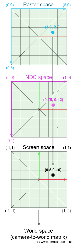
代码如下：

由于y是从上往下的，而屏幕空间的y是从下往上的，要将代码中的y乘以-1。

1
2
3

float x = (2 * ((i + 0.5) / scene.width) - 1) * scale * imageAspectRatio;
float y = (1 - 2 * (j + 0.5) / scene.height) * scale;
Vector3f dir = normalize(Vector3f(x, y, -1)); // Don't forget to normalize this direction!

使用fopen函数需要在属性->C/C++->预处理器->预处理器定义中添加以下宏_CRT_SECURE_NO_WARNINGS

Moller-Trumbore 算法

只要对着之前的公式敲就可以了，要注意的是判断浮点数相等的非常不准确的一件事情，由于相交的条件为t>=0，正确的写法是加上一个eps，即tnear + epsilon > 0。

bool rayTriangleIntersect(const Vector3f& v0, const Vector3f& v1, const Vector3f& v2, const Vector3f& orig,
                          const Vector3f& dir, float& tnear, float& u, float& v)
{
    // TODO: Implement this function that tests whether the triangle
    // that's specified bt v0, v1 and v2 intersects with the ray (whose
    // origin is *orig* and direction is *dir*)
    // Also don't forget to update tnear, u and v.

    Vector3f E1 = v1 - v0;
    Vector3f E2 = v2 - v0;

    Vector3f S = orig - v0;
    Vector3f S1 = crossProduct(dir, E2);
    Vector3f S2 = crossProduct(S, E1);
    
    tnear = dotProduct(S2, E2) / dotProduct(S1, E1);
    u = dotProduct(S1, S) / dotProduct(S1, E1);
    v = dotProduct(S2, dir) / dotProduct(S1, E1);

    float epsilon = 0.00001;
    if (tnear + epsilon > 0 && u + epsilon > 0 && v + epsilon > 0 && 1 - u - v + epsilon > 0)
        return true;

    return false;
}

最终结果如图：

加速结构

由于简单的计算光线与每个三角面相交非常慢，所以引入了加速计算光线追踪的算法。

Bounding Volumes

包围盒的思想是，如果光线不与包围盒相交，那么他也不会和包围盒内的三角面相交。这样可以大大减少计算的次数。一般我们使用AABBs即轴对齐包围盒。

二维情况下光线与AABB求交：

Ray AABB intersection

一个盒子（3D）= 三对无限大的平面

主要思想
- 射线只有在穿越所有平面对时才进入盒子
- 射线只要穿越任何一对平面就会离开盒子
对于每一对平面，计算t_min和t_max（负值也可以）
对于3D盒子，t_enter = max{t_min}，t_exit = min{t_max}
如果t_enter < t_exit，我们知道射线在盒子内停留一段时间（所以它们必定相交）

AABB判断求交的条件：
$$
t_{enter} < t_{exit} \ && \ t_{exit} >=0
$$

轴对齐包围盒求t的好处：

Uniform grids - 均匀网格

将空间划分成均匀的AABBs，网格的数量cells = C * objs，C ≈ 27 in 3D。

空间划分 - Spatial patitions

Oct-Tree（八叉树）
KD-Tree
BSP-Tree

但是KD-Tree很难写算法来判断物体是否跟AABB相交，因此很少用这种算法。

物体划分 - Object Partitions Bounding Volume Hierarchy（BVH）

这是工业界最常用的方法

建立一个BVH的过程如下：

寻找边界框
递归地将一组对象分成两个子集
重新计算子集的边界框
在必要（三角面少于一定数量）时停止
在每个叶子节点中存储对象

涉及到快速选择算法，找到中位数量的三角面，使得分出来的三角面数量趋近平均，从而缩小查找树的深度，减小搜索时间。

BVH（Bounding Volume Hierarchy）的数据结构

内部节点存储
- 边界框
- 子节点：指向子节点的指针
叶子节点存储
- 边界框
- 对象列表
节点表示场景中原语的子集
- 子树中的所有对象

BVH实现的伪代码：

作业6

目标

Ray-Bounding Volume包围盒求交：正确实现光线与包围盒求交函数。
BVH 查找：正确实现 BVH 加速的光线与场景求交

补充框架

Render() in Renderer.cpp:

框架里面已经计算了x和y，因此我们只需要补充剩下的生成光线的步骤即可，代码如下：

1 2	Vector3f dir = normalize(Vector3f(x, y, -1)); framebuffer[m++] = scene.castRay(Ray(eye_pos, dir), 0);

Triangle::getIntersection in Triangle.hpp:

这段代码初看没什么头绪，参考了以下文档：https://blueflame.org.cn/archives/437

这段代码需要补充的地方是给inter赋值，代码如下：

inline Intersection Triangle::getIntersection(Ray ray)
{
    Intersection inter;

    if (dotProduct(ray.direction, normal) > 0)
        return inter;
    double u, v, t_tmp = 0;
    Vector3f pvec = crossProduct(ray.direction, e2);
    double det = dotProduct(e1, pvec);
    if (fabs(det) < EPSILON)
        return inter;

    double det_inv = 1. / det;
    Vector3f tvec = ray.origin - v0;
    u = dotProduct(tvec, pvec) * det_inv;
    if (u < 0 || u > 1)
        return inter;
    Vector3f qvec = crossProduct(tvec, e1);
    v = dotProduct(ray.direction, qvec) * det_inv;
    if (v < 0 || u + v > 1)
        return inter;
    t_tmp = dotProduct(e2, qvec) * det_inv;

    // TODO find ray triangle intersection
    if (t_tmp < 0)
        return inter;
    inter.distance = t_tmp;//光线经过的时间
    inter.happened = true;//是否与三角形相交
    inter.m = m;//三角形的材质
    inter.obj = this;//Triangle继承了Object，重写了virtual Intersection getIntersection(Ray _ray)，三角形调用getIntersection(Ray _ray)，intersection自然记录下当前在相交的三角形，所以用this
    inter.normal = normal;//三角形面的法线
    inter.coords = ray(t_tmp);//Vector3f operator()(double t) const{return origin+direction*t;} in Ray.hpp, coords表示相交点的坐标

    return inter;
}

Ray-Bounding Volume包围盒求交

如果包围盒没有算好，可能会出现全蓝的错误结果。

在Bounds3.hpp中的IntersectP方法中，我们需要根据t_enter和t_exit直接的大小关系返回是否与该包围盒相交。

对于3D盒子，t_enter = max{t_min}，t_exit = min{t_max}，因此我们只需要求出xyz三对面的t_min和t_max即可，而三对面的t_min和t_max可以用轴对齐包围盒求t公式求解。

对于平行与x轴的面，公式如下：
$$
t = \frac{p’_x - o_x}{d_x}
$$
其他公式由此类推即可，以下是运行耗时14s的代码：

inline bool Bounds3::IntersectP(const Ray& ray, const Vector3f& invDir,
                                const std::array<int, 3>& dirIsNeg) const
{
    // invDir: ray direction(x,y,z), invDir=(1.0/x,1.0/y,1.0/z), use this because Multiply is faster that Division
    // dirIsNeg: ray direction(x,y,z), dirIsNeg=[int(x>0),int(y>0),int(z>0)], use this to simplify your logic
    // TODO test if ray bound intersects
    
    double t_enter = std::numeric_limits<double>::lowest();
    double t_exit = std::numeric_limits<double>::max();

    //对三对面进行判断
    for (int i = 0; i < 3; i++)
    {
        auto t_min = (pMin[i] - ray.origin[i]) * invDir[i];
        auto t_max = (pMax[i] - ray.origin[i]) * invDir[i];
        if (!dirIsNeg[i])
            std::swap(t_min, t_max);

        t_enter = std::max(t_min, t_enter);
        t_exit = std::min(t_max, t_exit);
    }

    float eps = 0.00001;
    if (t_enter < t_exit && t_exit + eps > 0)
        return true;
    else
        return false;
}

以下是运行耗时2min的代码：

inline bool Bounds3::IntersectP(const Ray& ray, const Vector3f& invDir,
                                const std::array<int, 3>& dirIsNeg) const
{
    // invDir: ray direction(x,y,z), invDir=(1.0/x,1.0/y,1.0/z), use this because Multiply is faster that Division
    // dirIsNeg: ray direction(x,y,z), dirIsNeg=[int(x>0),int(y>0),int(z>0)], use this to simplify your logic
    // TODO test if ray bound intersects
    
    double t_enter = std::numeric_limits<double>::lowest();
    double t_exit = std::numeric_limits<double>::max();

	auto x_min = (pMin.x - ray.origin.x) * invDir[0];
	auto x_max = (pMax.x - ray.origin.x) * invDir[0];
	if (!dirIsNeg[0])
    	std::swap(x_min, x_max);

	auto y_min = (pMin.y - ray.origin.y) * invDir[1];
	auto y_max = (pMax.y - ray.origin.y) * invDir[1];
	if (!dirIsNeg[1])
    	std::swap(y_min, y_max);

	auto z_min = (pMin.z - ray.origin.z) * invDir[2];
	auto z_max = (pMax.z - ray.origin.z) * invDir[2];
	if (!dirIsNeg[2])
    	std::swap(z_min, z_max);

	t_enter = std::max(x_min, std::max(y_min, z_min));
	t_exit = std::min(x_max, std::max(y_max, z_max));
    
    float eps = 0.00001;
    if (t_enter < t_exit && t_exit + eps > 0)
        return true;
    else
        return false;
}

BVH 查找

根据之前的伪代码写以下的代码即可

需要注意，IntersectP里面的参数有一项 const std::array<int, 3>& dirIsNeg，需要用以下格式输入：

{ray.direction.x > 0, ray.direction.y > 0, ray.direction.z > 0}

Intersection BVHAccel::getIntersection(BVHBuildNode* node, const Ray& ray) const
{
    // TODO Traverse the BVH to find intersection

    if (node->bounds.IntersectP(ray, ray.direction_inv, {ray.direction.x > 0, ray.direction.y > 0, ray.direction.z > 0}))
    {
        if (node->left == nullptr && node->right == nullptr)
        {
            return node->object->getIntersection(ray);
        }
        else
        {
            auto hit1 = getIntersection(node->left, ray);
            auto hit2 = getIntersection(node->right, ray);
            return hit1.distance < hit2.distance ? hit1 : hit2;
        }
    }
    return Intersection();
}

结果如图：

辐射度量学 - Radiometry

之前做的Blinn-Phong光照模型只描述了光I的强度，不能很好的表示光，所以需要一个能够精确定义光的项。

辐射度量学精确地定义了光，能够描述光的属性（空间）

Radiant flux
intensity
irradiance
radiance

基本物理量

Radiant：

能量，但是基本不用这个。

$$
Q[J=Joule]
$$

Radiant Flux(Power)：

由于在图形学中，我们知道物体受光照越长，吸收能量越多，所以我们更喜欢用单位时间的能量（功率）。

$$
\Phi = \frac{dQ}{dt}
$$

Intensity：

一个立体角上的能量

$$
I = \frac{\Phi}{4\pi}
$$

Solid Angle:

立体角，对于不同的物体，把它投影到单位球上（与单位球球心连线），会框出一个范围，这就是立体角。

$$
\Omega = \frac{A}{r^2}
$$

Irradiance:

单位面积的能量，面要与光线垂直。

$$
E(x) = \frac{d \Phi (x)}{dA}
$$

Irradiance和Blinn-Phong光照模型中的兰伯特余弦定理的关系：

从下面这张图可以看出，Irradiance是在衰减的，而Intensity不会衰减，是因为Intensity随着传播距离的增大，对应的面积也会增大，结果是Intensity保持不变的。

Radiance:

为了描述光在直线上传播的引入属性，非常重要，与路径传播有关。

Radiance是在单位立体角，在单位投影面积上的能量。

$$
L(p, \omega) \equiv \frac{d^2 \Phi(p, \omega) }{d\omega \ dA \cos\theta }
$$

Irradiance和Radiance能够告诉我们物体是如何反射光。

Bidirectional Reflectance Distribution Function(BRDF) - 双向反射分布函数

接受Irradiance

输出Radiance

BRDF项定义了不同的材质。

反射光可以等于所有入射到某个点的入射光经过反射的积分，这就是反射方程

反射方程加上能量产生项就能得到渲染方程

渲染方程通过算子的方式可以展开得到不同的光线经过反射得到的次数

0次是光源本身，1次是直接光照，2次或更多就是间接光照

直接光照加上间接光照就是全局光照

光线传播

The reflect equation 反射方程

The rendering equation 渲染方程

渲染方程描述了光线传播，它是由一个自发光项和反射方程组成。

概率论复习

随机变量

连续情况下如何描述概率

连续性随机变量

概率密度

蒙特卡洛积分

给定任何一个函数，我们想算它从a到b的定积分，如果这个函数比较复杂，我们不希望写出解析式就能得出定积分的结果，就可以用蒙特卡洛方法解定积分。

路径追踪

我们已经学过了Whitted-Style Ray Tracing，但他有很多问题需要优化。

以下是Whitted-Style Ray Tracing的问题：

对于Glossy反射的效果不对（正确的Glossy反射也会有一点Specular反射）
漫反射物体之间没有反射

Blinn-Phong光线方向向外

两个问题：指数爆炸、递归边界

路径最终不好处理点光源。

作业7

目标

迁移代码
Path Tracing：正确实现 Path Tracing 算法
（附加题）多线程：将多线程应用在 Ray Generation 上
（附加题）Microfacet：正确实现 Microfacet 材质

迁移代码

Triangle.hpp:

inline Intersection Triangle::getIntersection(Ray ray)
{
    Intersection inter;

    if (dotProduct(ray.direction, normal) > 0)
        return inter;
    double u, v, t_tmp = 0;
    Vector3f pvec = crossProduct(ray.direction, e2);
    double det = dotProduct(e1, pvec);
    if (fabs(det) < EPSILON)
        return inter;

    double det_inv = 1. / det;
    Vector3f tvec = ray.origin - v0;
    u = dotProduct(tvec, pvec) * det_inv;
    if (u < 0 || u > 1)
        return inter;
    Vector3f qvec = crossProduct(tvec, e1);
    v = dotProduct(ray.direction, qvec) * det_inv;
    if (v < 0 || u + v > 1)
        return inter;
    t_tmp = dotProduct(e2, qvec) * det_inv;

	if (t_tmp < 0)
		return inter;

    // TODO find ray triangle intersection
    inter.distance = t_tmp;//光线经过的时间
    inter.happened = true;//是否与三角形相交
    inter.m = m;//三角形的材质
    inter.obj = this;//Triangle继承了Object，重写了virtual Intersection getIntersection(Ray _ray)，三角形调用getIntersection(Ray _ray)，intersection自然记录下当前在相交的三角形，所以用this
    inter.normal = normal;//三角形面的法线
    inter.coords = ray(t_tmp);//Vector3f operator()(double t) const{return origin+direction*t;} in Ray.hpp, coords表示相交点的坐标

    return inter;
}

加了这一条，没有黑点了
if (t_tmp < 0)
    return inter;

Bounds3.hpp

inline bool Bounds3::IntersectP(const Ray& ray, const Vector3f& invDir,
                                const std::array<int, 3>& dirIsNeg) const
{
    // invDir: ray direction(x,y,z), invDir=(1.0/x,1.0/y,1.0/z), use this because Multiply is faster that Division
    // dirIsNeg: ray direction(x,y,z), dirIsNeg=[int(x>0),int(y>0),int(z>0)], use this to simplify your logic
    // TODO test if ray bound intersects
    double t_enter = std::numeric_limits<double>::lowest();
    double t_exit = std::numeric_limits<double>::max();

    //对三对面进行判断
    for (int i = 0; i < 3; i++)
    {
        auto t_min = (pMin[i] - ray.origin[i]) * invDir[i];
        auto t_max = (pMax[i] - ray.origin[i]) * invDir[i];
        if (!dirIsNeg[i])
            std::swap(t_min, t_max);

        t_enter = std::max(t_min, t_enter);
        t_exit = std::min(t_max, t_exit);
    }

    if (t_enter <= t_exit && t_exit >= 0)
        return true;
    else
        return false;
}

BVH.cpp

Intersection BVHAccel::getIntersection(BVHBuildNode* node, const Ray& ray) const
{
    // TODO Traverse the BVH to find intersection
    if (node->bounds.IntersectP(ray, ray.direction_inv, { ray.direction.x > 0, ray.direction.y > 0, ray.direction.z > 0 }))
    {
        if (node->left == nullptr && node->right == nullptr)
        {
            return node->object->getIntersection(ray);
        }
        else
        {
            auto hit1 = getIntersection(node->left, ray);
            auto hit2 = getIntersection(node->right, ray);
            return hit1.distance < hit2.distance ? hit1 : hit2;
        }
    }
    return Intersection();
}

Path Tracing 算法

以下是作业pdf中的伪代码：

shade (p, wo)
    sampleLight (inter , pdf_light)
    Get x, ws , NN , emit from inter
    Shoot a ray from p to x
    If the ray is not blocked in the middle
        L_dir = emit * eval(wo , ws , N) * dot(ws , N) * dot(ws , NN) / |x-p|^2 / pdf_light
    
    L_indir = 0.0
    Test Russian Roulette with probability RussianRoulette
    wi = sample (wo , N)
    Trace a ray r(p, wi)
    If ray r hit a non - emitting object at q
        L_indir = shade (q, -wi) * eval (wo , wi , N) * dot(wi , N) / pdf(wo , wi , N) / RussianRoulette
    
    Return L_dir + L_indir

根据作业pdf中的伪代码敲：

Vector3f Scene::castRay(const Ray &ray, int depth) const
{
    // TO DO Implement Path Tracing Algorithm here
    Intersection intersection = intersect(ray);

    //没有碰到物体，而是碰到背景的情况
    if (!intersection.happened)
    {
        return Vector3f(0);
    }

    //打到光源的情况，说明只计算自发光项
    if (intersection.m->hasEmission())
    {
        if (depth == 0)
            return intersection.m->getEmission();
        else
            return Vector3f(0);
    }

    // 射到物体的情况
    Vector3f L_dir(0), L_indir(0);

    //对场景中的光源均匀采样，得到pdf
    Intersection inter_light;
    float pdf = 0.f;
    sampleLight(inter_light, pdf);

    Vector3f p = intersection.coords;
    Vector3f x = inter_light.coords;
    Vector3f wo = ray.direction;
    Vector3f ws = (x - p).normalized();
    Vector3f N = intersection.normal.normalized();
    Vector3f NN = inter_light.normal.normalized();
    Vector3f emit = inter_light.emit;
    float distance = (x - p).norm();

    //从p点向x点射出光线
    //修正的p点
    Vector3f fixed_p = (dotProduct(ray.direction, N) < 0) ?
        p + N * EPSILON :
        p - N * EPSILON;

    Ray ray_p2x(fixed_p, ws);

    //由p点射出的光线相交的距离小于光线的距离，说明被物体遮挡，需要计算直接光照
    if ((intersect(ray_p2x).distance - distance > -0.0001))
    {
        L_dir = emit * intersection.m->eval(wo, ws, N) * dotProduct(ws, N) * dotProduct(-ws, NN) / (distance * distance) / pdf;
    }

    //俄罗斯轮盘赌
    if (get_random_float() < RussianRoulette)
    {
        //计算间接光照
        Vector3f wi = intersection.m->sample(wo, N).normalized();
        Ray nextRay(fixed_p, wi);
        Intersection nextInter = intersect(nextRay);
        if (nextInter.happened && !nextInter.m->hasEmission())
        {
            L_indir = castRay(nextRay, depth + 1) * intersection.m->eval(wo, wi, N) * dotProduct(wi, N) / intersection.m->pdf(wo, wi, N) / RussianRoulette;
        }
    }

    return L_dir + L_indir;
}

关于p点的问题：https://zhuanlan.zhihu.com/p/606074595

需要注意的是：

从p点向x点射出光线，需要对p点进行修正，否则会出现不正确的阴影
直接光照的判断条件中，需要将eps调大，否则会出现黑边

需要注意的是，p点要修正，否则会产生以下的错误结果：

随机数问题

随机数构造器优化：https://zhuanlan.zhihu.com/p/606074595

C++的性能分析器：https://blog.csdn.net/u011942101/article/details/123656944

在global.hpp中将以下三个变量设置为static，能够加速图像的生成。由于这个函数频繁地被调用，其中的变量经常被反复构建，造成了很大性能开销。将这些变量设置为static，那么这些变量只会初始化一次，避免了重复构建。

inline float get_random_float()
{
    static std::random_device dev;
    static std::mt19937 rng(dev());
    static std::uniform_real_distribution<float> dist(0.f, 1.f); // distribution in range [1, 6]

    return dist(rng);
}

多线程

C++多线程教程：https://blog.csdn.net/sjc_0910/article/details/118861539

以下是实现多线程需要注意的地方：

可以将渲染像素的过程使用lambda表达式写出来，这样能够方便地使用多线程。
UpdateProgress这个函数可能会造成冲突，需要上锁

void Renderer::Render(const Scene& scene)
{
    std::vector<Vector3f> framebuffer(scene.width * scene.height);

    float scale = tan(deg2rad(scene.fov * 0.5));
    float imageAspectRatio = scene.width / (float)scene.height;
    Vector3f eye_pos(278, 273, -800);

    //开启多线程
    int numThreads = std::thread::hardware_concurrency();
    std::vector<std::thread> threads(numThreads);
    std::mutex mutex;
    int process = 0;
    int rowsPerThread = scene.height / numThreads;

    // change the spp value to change sample ammount
    int spp = 16;
    std::cout << "SPP: " << spp << "\n";

    //将渲染每个像素的过程封装到一个函数中，其中捕获列表捕获当前作用域内所有变量，引用传递
    auto renderPixel = [&](uint32_t startRow, uint32_t endRow) {
        //m是像素数组的下标，由于多线程是随机的，因此需要在每次运行前判断当前的m
        int m = startRow * scene.width;
        for (uint32_t j = startRow; j < endRow; ++j) {
            for (uint32_t i = 0; i < scene.width; ++i) {
                // generate primary ray direction
                float x = (2 * (i + 0.5) / (float)scene.width - 1) *
                    imageAspectRatio * scale;
                float y = (1 - 2 * (j + 0.5) / (float)scene.height) * scale;

                Vector3f dir = normalize(Vector3f(-x, y, 1));
                for (int k = 0; k < spp; k++) {
                    framebuffer[m] += scene.castRay(Ray(eye_pos, dir), 0) / spp;
                }
                m++;
            }
            //需要对这个操作进行上锁，防止冲突
            mutex.lock();
            UpdateProgress(++process / (float)scene.height);
            mutex.unlock();
        }
    };

    //使用多线程执行renderPixel函数
    for (int t = 0; t < numThreads; ++t) {
        threads[t] = std::thread(renderPixel, t * rowsPerThread, (t + 1) * rowsPerThread);
    }

    // 等待所有线程完成
    for (int i = 0; i < numThreads; ++i) {
        threads[i].join();
    }  

    UpdateProgress(1.f);

    // save framebuffer to file
    FILE* fp = fopen("binary.ppm", "wb");
    (void)fprintf(fp, "P6\n%d %d\n255\n", scene.width, scene.height);
    for (auto i = 0; i < scene.height * scene.width; ++i) {
        static unsigned char color[3];
        color[0] = (unsigned char)(255 * std::pow(clamp(0, 1, framebuffer[i].x), 0.6f));
        color[1] = (unsigned char)(255 * std::pow(clamp(0, 1, framebuffer[i].y), 0.6f));
        color[2] = (unsigned char)(255 * std::pow(clamp(0, 1, framebuffer[i].z), 0.6f));
        fwrite(color, 1, 3, fp);
    }
    fclose(fp);    
}

效果提升显著，从18分钟缩减到1分钟。

问题

渲染结果较暗，出现横向黑色条纹的情况，很可能是因为直接光部分由于精度问题，被错误判断为遮挡，请试着通过精度调整放宽相交限制。

解决方法：增大直接光照判断条件中的eps。
渲染结果全黑或几乎全黑，右边完全看不见物体，是因为包围盒AABB的判断错误，天花板和周围的面是没有厚度的，这导致在判断的时候没有纳入相交。

解决方法：需要考虑t_enter == t_exit的情况

材质与外观

光线与材质之间的作用形成了不同的外观

在渲染方程中，BRDF项决定了材质如何被反射，是用来定义材质的项。

也就是说，Material == BRDF

BSDF = BRDF + BTDF

本章介绍了以下不同的材质：

Diffuse / Lambertian Material (BRDF)
Glossy material (BRDF)
Ideal reflective / refractive material (BSDF*)
Fresnel Reflection / Term

Reflectance depends on incident angle (and polarization of light)
- 使用Schlick’s近似
Microfacet Material - 微表面材质，基于物理的材质

从远程看看到的是材质，从近处看看到的是几何
Isotropic / Anisotropic Materials (BRDFs)

区分材质的方法：各项同性、各向异性。各项同性：微表面（法线）不存在方向性，各向异性的微表面存在方向性。

BRDFs的属性

非负，因为代表能量的分布
线性，可以拆成很多块加起来
可逆性，交换入射方向和出射方向，得到的BRDF还是一样的
能量守恒，入射能量积分小于等于1（表现为全局光照迭代一定次数后会收敛）
各向异性和各向同性

测量BRDFs

MERL BRDF Database

高级光线传播与复杂外观建模

高级光线传播

高级光线传播的方法包括以下几种：

无论使用多少样本，无偏估计的期望值将始终是正确的值，否则就是有偏。

有偏估计有一个特殊的方法，期望值在使用无限数量的样本时趋于正确值

无偏光线传播方法
- Path Tracing（工业界最常用的方法，最稳定）
- BDPT
- MLT
有偏光线传播
- Photon Mapping - 光子映射
- Vertex connection and merging (VCM) - 顶点连接与合并
Instant radiosity (VPL / many light methods) - 实时辐射度算法

Bidirectional Path Tracing (BDPT) - 双向路径传播

通过实现一条连接相机和光线的路径实现光线追踪。同时跟踪来自相机和光源的子路径，并连接连接来自两个子路径的端点。

适用于较复杂光源情况，但是难以实现并且计算缓慢。

Metropolis Light Transport(MLT)

马尔科夫链：通过某些概率密度函数（PDF）从当前样本跳转到下一个样本

应用了马尔科夫链，当f(x)和p(x)相似也就是采样函数和被积函数形状相似的时候，能够得到更好的variance，能够在复杂光线路径下得到较好的结果，比如在场景中全是间接光照的时候。

关键思想：局部通过局部扰动现有路径以获得新路径

但是MLT无法预测收敛速度，无法知道什么时候降噪效果最好，因此得出来结果很脏，无法用来渲染动画。

Photon Mapping - 光子映射

特别用来渲染caustics的方法，是一个两阶段的方法

第一阶段 — 光子追踪
- 从光源发射光子，让它们反射，然后记录在漫反射表面上的光子
第二阶段 — 光子收集（最终合成）
- 从相机发射子路径，让它们反射，直到它们击中漫反射表面
计算 — 局部密度估计
- 思想：拥有更多光子的区域应该更亮
- 对于每个着色点，找到最近的N个光子。考虑它们所覆盖的表面积

一个例子可以让你更容易理解渲染中的偏差

有偏差 == 模糊

一致的 == 使用无限数量的样本不会模糊

Vertex Connection and Merging

结合了BDPT和Photon Mapping的方法

主要思想：

如果BDPT中的子路径的终点无法连接但可以合并，就不要浪费它们
使用光子映射来处理附近“光子”的合并

Instant Radiosity (IR)

有时也称为“多光源方法”

主要思想是将可以被照亮的表面被视为光源

实现方法：

在表面上发射光子子路径，假设每个子路径的终点是虚拟点光源（VPL）
使用这些VPL正常渲染场景

优点：

在漫反射场景上运行速度快，通常能产生良好的结果

缺点：

当VPL接近着色点时，可能会出现突亮的点
无法处理Glossy材质

复杂外观建模

包含以下课题：

Non-surface models
- Participating media
- Hair / fur / fiber (BCSDF)
- Granular material
Surface models
- Translucent material (BSSRDF) - 次表面散射材质
- Cloth
- Detailed material (non-statistical BRDF)
Procedural appearance

Non-surface models

Participating media - 散射介质

像雾、云这一类没有实体的都是散射介质，在光线穿过散射介质时，它可以（部分地）被吸收和散射。

这类介质在反射时不一定都像漫反射一样均匀地向四周发射，因此使用相函数来描述在参与介质内任意点x处的光散射的角分布。

渲染的实现：

随机选择一个方向进行反射
随机选择一个距离直线前进
在每个“着色点”处，连接到光源

Hair / fur / fiber (BCSDF)

Marschner Model

这个模型描述了每一根头发跟光线的作用，Marschner Model将头发看作是玻璃一样的圆柱体，光线通过这个圆柱体会发生R、TT、TRT三种反射。

Double Cylinder Model

由于Marschner Model对于动物毛发的效果不是很好，表现为不是很亮，因此根据真实的毛发结构提出了这个模型。

相较于Marschner Model，Double Cylinder Model主要是增加了Medulla这一项

除了会发生R、TT、TRT三种反射，Double Cylinder Model还会发生TTs，TRTs反射。

Granular material

可以被翻译为颗粒材质，通过程序定义可以避免明确建模所有颗粒。

Surface models

Translucent material (BSSRDF) - 次表面散射材质

BSSRDF：BRDF的泛化；由另一点的入射微分辐照度而得到的一点处的出射辐亮度。对于渲染方程：在表面上的所有点和所有方向上进行积分

一般使用引入两个点光源来近似次表面散射。

cloth - 布料渲染：

布料是由许多的纤维（Fibers）组成股（Ply），然后由许多的Ply组成线（Yarn），将Yarn通过织造（Woven）或者针织（Knitted）的方法织成衣服。

主要通过三种方式实现渲染：散射介质、实际纤维、物体表面

Detailed - 细节渲染

动机：渲染出来的东西不真实，实际上真实的物体在强光照射下有划痕

从法线的贡献度出发，现实中的法线形似但和像理论中的法线一样规整。

近年来的研究趋势：波动光学

Procedural appearance

我们可以定义细节而不用使用材质贴图，通过计算噪声函数，每次需要只要通过查询就能得到细节。

这个领域比较前沿的研究有3DsMax的木制贴图。

相机与透镜

目前图形学有两种成像方法：光栅化和光线追踪，它们都是合成的方法。

最早对相机的研究：小孔成像

相机的部件：

快门：控制光在一定时间内进入相机
传感器：记录进入的光线，上面的每个点记录的是Irradiance

光线追踪用的也是针孔相机的模型，因此做不出带有景深的渲染

Field of View（FOV）

传感器增大，FOV也会增大

Exposure - 曝光

曝光是由三个参数进行控制的：

Aperture size（光圈大小）
- 通过改变F-Stop（F-Number）来打开/关闭光圈（如果相机具有光圈控制）来改变光圈大小
- f数越小，对应光圈越大
Shutter speed（快门速度）
- 改变传感器内像素的光线持续的时间
- 快门速度越快，进到传感器的光越少
ISO gain（感光度增益）
- 改变传感器值与数字图像值之间的放大（模拟和/或数字放大）

ISO

可以理解成后期处理，不改变传感器最终接受到多少能量，而是将这个能量乘以一个数使得亮度变大。但是ISO拉大亮度的同时会增大噪声。

快门速度

把光看出是光子，当增大快门速度，进到感光元件的光子就少，得到的图片会比较暗。曝光时间越长，运动模糊越严重。物体运动的速度和快门速度接近或者快的时候，相机获取到不同时间下的物体位置就会产生扭曲。

快门速度和光圈的关系：

快门速度高，调小光圈，常用于高速摄影
快门速度低，运动模糊严重，常用在延迟摄影

运动模糊也不都是坏的，当你需要描述一个高速物体的时候使用运动模糊就能很好的表示速度感。

光圈

下图表示的是调整光圈和快门速度得到相同曝光的参数：

如果想要景深就没有运动模糊，如果想要运动模糊就没有景深

薄透镜近似

现代的相机能实现变焦是因为它们是有透镜组组成的。

理想化的薄棱镜模型中，光线会聚焦到同一个点。

其中，zo是物距，zi是相距。

Defocus Blur

CoC用来描述焦点之外的物体在成像平面上呈现为模糊圆形的现象。当一点或一个物体不在焦点上时，它的光线不会准确地汇聚在成像平面上的单一点上，而是会在周围形成一个小圆圈。

CoC和光圈大小是成正比的，增大光圈也增大了CoC，景深程度也会增大。

Ray Tracing Ideal Thin Lenses

设置：

选择传感器尺寸、镜头焦距和光圈大小
选择感兴趣的主题深度zo
通过薄透镜方程计算相应的传感器深度zi

渲染过程：

对于传感器（实际上是胶卷）上的每个像素x’来说，
在镜头平面上采样随机点x’’，
通过镜头的射线将会击中x’’’（因为x’’’在焦点内，考虑虚拟射线（x’，镜头中心）），
估计射线x’’ -> x’’’上的辐射度。

Depth of Field

景深是指呈像清晰的一段距离，景深锐利的地方都是CoC小的地方

光场、颜色与感知

光场

Light Field - 光场：是一个四维的分布uvst，空间中任何一个点可以记录的光线的强度

The Plenoptic Function(全光函数)：我们能看到的所有事物的集合

$$
P(\theta, \phi. \lambda, t, V_X, V_Y, V_Z)
$$
其中θ和Φ觉得了可视角度；λ决定了光线的强度即颜色；t决定了时间，引入t就是类似于电影的概念；VxVyVz能够得到任何位置的视点，类似于全息电影。

可以用一个立方体的表面保存由于所包围的对象而产生的所有radiance

知道uvst四个点的信息就能知道光线的位置和方向。

光场相机

能够后期重新聚焦、处理照片的相机，因为他传感器后置，原本传感器的位置是一个精密的棱镜，棱镜将光线分成很多份，后置的传感器每个像素使用更大的规格来存储这些被分离的光线。

物理角度下的颜色

颜色是人的感知现象，它不是光的属性，不同波长的光不是“颜色”。一般我们探讨的的颜色是我们感知到的可见光。

SPD：可以用描述光在不同波长上的分布，SPD有线性的性质，可以相加。

人眼的构造：

瞳孔：控制进光量，相当于光圈
晶状体：相当于透镜
视网膜：相当于传感器，最终光线到达的地方

视网膜内的感光细胞：
- Rods - 棒状细胞：用来感知光线的强度，灰度图
- Cones - 锥形细胞：用来感知颜色
  - S,M,L分别感知低、中、高波长的光

Metamerism （同⾊异谱）

同色异谱是指将现实中的光谱投射到（S,M,L）三维响应曲线上，使其在人类感知上是一样的。

这多用来做色彩匹配 - color matching

在计算机中，大多都是用加色系统进行色彩匹配，比如RGB，颜色会越加越亮。在印刷行业大多是用减色系统，颜色会越加越黑。

色彩空间

为了可视化色域图，将XYZ映射到两维，通过归一化并且固定Y，得到相同亮度下的颜色值，也就是色域。

其他色彩空间有：HSV、Lab，减色系统的色彩空间有：CMYK，基于成本考虑，一般不会用三种颜色混合出黑色，而是直接用黑色墨水。不同颜色空间的色域范围不同。

互补色理论

由于人脑有颜色暂留的机制，能够自动补全，所以才有了互补色的理论。当长时间盯着一张图，切换的时候会显示出它的互补色。

感知和联系有关

一个被津津乐道的例子是两个灰度图，看起来亮度不同，但是把周围的影响的环境因素遮住后灰度其实是一样的。

动画与模拟

Introduction to Computer Animation

History
Keyframe animation
Physical simulation
Kinematics
Rigging

动画中，美学通常主导技术。在3D中，动画也可以看作是建模的延伸：将模型表示为时间的函数。

在不同媒介中对帧数的要求：

Film: 24 frames per second
Video (in general): 30 fps
Virtual reality: 90 fps

Keyframe Animation

Animator 创建关键帧
Assistant (person or computer) 创建中间帧

在中间帧之间使用线性插值通常没有很好的效果，因此通过应用样条（曲线）生成平滑的插值。

物理模拟

通过建立物理正确的模型，就能模拟物理效果

例子：

头发模拟
网格模拟
粒子模拟
布料模拟

Mass Spring System - 质点弹簧系统

质点弹簧系统是一系列相互连接的质点和弹簧组成的系统。

假设a和b两个质点之间有一条长度为l的弹簧，可以通过以下式子表示它们之间力的关系。

b-a是b到a的向量。

能量损失

由于该系统没有能量损失，会不断的在弹性势能和动能之间振动转换，就会不停地弹下去。为了避免这种情况，引入了energy loss。

使用Damping用来表示内部的损耗，表现得像运动中的粘滞阻力，通过减缓速度方向的运动来损耗能量，其中 kd 是阻尼系数。

在物理模拟中，b一点和a一点表示速度，两点表示为加速度。

Structures from Springs

添加通过斜向之间的作用力（蓝线）来抵抗切变，通过使用skip connection（红线）来抵抗平面外弯曲力类似于将平面对折之间的阻力。红线的力要比蓝线的力小。

另外一个模拟布料的方法：有限元方法，是通过模拟力传导、热传导这些扩散现象模拟布料。

Particle Systems - 粒子系统

粒子系统的思想是计算一个集合中的每个粒子的运动来模拟动画，是图形学和游戏中比较流行的技术。

它的实现比较容易，可扩展性强（性能差时使用较少的粒子，复杂性较高时使用更多的粒子）

面临的挑战：可能需要许多粒子（例如流体）、可能需要加速结构（例如查找相互作用的最近粒子）

粒子系统的实现过程：

[If needed] Create new particles
Calculate forces on each particle
Update each particle’s position and velocity
[If needed] Remove dead particles
Render particles

除了粒子自己存在的速度之外，粒子和粒子之间或者粒子和其他物体之间也有作用力：

吸引力和排斥力

重力、电磁力、…
弹簧、推进力、…

阻尼力

摩擦、空气阻力、粘度、…

碰撞

墙壁、容器、固定物体、…
动态物体、角色身体部位、…

复杂粒子

个体与群体之间的关系，例如将每只鸟模拟为一个粒子。他们之间存在以下自发的力的作用：

吸引力：向邻居的中心的吸引力
排斥力：从单个邻居的排斥力
对齐：朝着邻居的平均轨迹的方向对齐

运动学

Forward Kinematics - 正向动力学

正向运动学实现容易，但是不方便艺术家调整，艺术家一般使用IK进行动画

使用骨骼去驱动模型，骨架包括以下结构：

关节骨架

拓扑结构（连接关系）
关节处的几何关系
树形结构（无环路的情况下）

关节类型

钉销关节（1D 旋转）
球关节（2D 旋转）
棱柱关节（平移）

通过记录时间t内每个骨骼的旋转位置可以保存这段时间的动画。

正向运动学的优缺点

优点：

直接控制方便
实施相对简单

缺点：

动画可能与物理不一致
耗时较长，对艺术家来说较为繁琐

Inverse Kinematics - 逆向运动学

动画师提供末端执行器的位置，应用计算出满足约束的关节角度。

但是这种方法存在很多问题需要解决：结果不唯一，或者无解

解决一般的N连杆逆运动学问题的数值方法：

选择初始配置
定义误差度量（例如，目标位置与当前位置之间的距离的平方）
计算误差关于配置的梯度
应用梯度下降（或牛顿法，或其他优化过程）

Rigging - 绑定

绑定（Rigging）绑定是对角色的一组高级控制，允许更快速和直观地修改姿势、变形、表情等。

重要特点：

像使用木偶的线一样控制角色
捕捉所有有意义的角色变化
因角色而异

绑定创建成本高昂，需要手工调整以及艺术和技术的结合。

Blend Shapes - 混合形状

不使用骨骼，直接在表面之间进行插值。例如，对面部表情进行建模。

最简单的方案：采用顶点位置的线性组合，使用样条控制随时间变化的权重选择

Motion Capture - 动作捕捉

动作捕捉是数据驱动的动画制作方法

记录现实世界的表演（例如，人执行某项活动）
从收集的数据中提取随时间变化的姿势

优点

能够快速捕获大量的真实数据
可以达到较高的逼真度

缺点

复杂且昂贵的设置
捕获的动画可能不符合艺术需求，需要进行修改

实现方案

光学

通过机器视觉的方法读取动捕演员身上的球状、片状控制点提取位置信息
通过高帧率如240HZ的摄像机拍摄多角度照片、影片
遮挡关系很难解决

磁性

感知磁场以推断位置/方向，有束缚性。

机械

直接测量关节角度，限制了运动的角度。

面部捕捉的挑战：恐怖谷效应。

动画生产管线

Single particle simulation

为了模拟粒子的运动，我们需要模拟某个粒子在速度场（能够知道任何位置在某一时刻的速度）中的情况。

随时间计算粒子位置需要解决一阶常微分方程（Ordinary Differential Equation，ODE），在实际的例子中，我们使用欧拉方法来计算。

常微分方程是不存在对其他变量的微分、导数，只有一个变量的微分方程

“常”表示没有“偏导数”，也就是 x 只是时间 t 的函数

显示欧拉方法 - Explicit Euler method

也称为Forward Euler，这种方法不是很准，需要用到较小的Δt才会更精准，很容易不稳定。

对于显示欧拉方法，有两个关键问题需要解决：

随着时间步长 Δt 的增加，不准确性也会增加。
不稳定性是一个常见且严重的问题，可能导致模拟发散（信号与系统中的正反馈，导致错误被放大）。

用数值方法解微分方程都会遇到的问题：

误差

在每个时间步长上，误差会逐渐积累，随着模拟的进行，准确度会下降
不过在图形应用中，准确性可能不是关键问题。

不稳定

误差可以累积，导致模拟发散，即使基础系统没有发散，导致和实际下物理情况差的特别远
稳定性不足是模拟中的一个基本问题，不能忽视。

Instability and improvement

以下是应对不稳定的改进方法：

中点法 - Modified Euler

在起点和终点处平均速度

动态步长法（自适应步长）

递归地比较一步和两个半步，直到误差可接受

隐式欧拉法（后向欧拉法）

使用未来时间的粒子的位置和速度

中点法 - Modified Euler

平均每一个步长中起点和终点的速度，能够得到比显示欧拉更好的效果。

动态步长法（自适应步长）

基于错误估计选择步长的技术，非常实用，但可能需要非常小的步长！

算法实现需要重复以下过程直到误差低于阈值：

计算 x_T ,一个大小为 T 的欧拉步骤
计算 x_T/2, 两个大小为 T/2 的欧拉步骤
计算误差 || xT – xT/2 ||
如果（误差 > 阈值）
减小步长并重试

隐式欧拉法（后向欧拉法）

使用下一时刻的导数用到当前的速度中。能够解决（x^t+Δt）和（ x点^t+Δt， x点是x一阶导）的非线性问题，同时也能提供更好的稳定性。

计算较困难，具体实现会使用寻根算法，例如牛顿法。

怎么定义/量化稳定性？

使用（局部误差）/（整体误差）
绝对值不重要，但相对于步长的阶数重要，阶数越高越好
隐式欧拉法是一阶的，这意味着：
- 局部误差O(h^2)
- 全局误差O(h)
O(h)的意义：
- 如果我们将h减半，我们可以期望误差也减半。
- O(h^2)中，如果减小一半h，误差减小1/4h，因此阶数越高越好。

Runge-Kutta Families

荣格库塔方法，是一系列的方法，这里介绍的是RK4算法，也是O(h^4)的一种算法。

信号处理，数值分析课会详细介绍荣格库塔方法

Position-Based / Verlet Integration

不是基于物理的方法，在模拟中非常好用。

思想：

使用中心欧拉法计算之后，限制粒子的位置以防止发散和不稳定行为
使用受限制的位置来计算速度
这两个想法都会耗散能量，稳定系统

优缺点：

快速和简单
不基于物理，会耗散能量（引入误差）

Rigid body simulation

刚体，不会发生形变，会让内部的所有的点按照相同的方向运动。能够模拟一个粒子子也能够模拟一个刚体，但是模拟刚增添一些额外的物理量：

位置 - 速度
角度（朝向） - 角速度
速度 - 加速度
角速度 - 角加速度

Fluid simulation

假设水是有很多小的rigid-body的球体组成，如何模拟这些球体的运动就能解决模拟流体的问题。

A Simple Position-Based Method：

关键思想

假设水由小的刚体球体组成
假设水不能被压缩（即密度恒定）
因此，只要密度在某处发生变化，它应该通过改变粒子的位置来“校正”
您需要知道密度相对于每个粒子的位置的梯度
更新？只需要梯度下降！

Eulerian vs. Lagrangian

质点法 - Lagrangian

网格法 - Eulerian

Material Point Method (MPM)

混合了质点法和网格法，先使用网格法进行数值分析，然后将结果插值回粒子。

作业8

实现要求：

连接绳子约束，正确的构造绳子
半隐式欧拉法
显式欧拉法
显式 Verlet
阻尼

你应该修改的函数是:

rope.cpp 中的 Rope::rope(…)
rope.cpp 中的 void Rope::simulateEuler(…)
rope.cpp 中的 void Rope::simulateVerlet(…)

环境配置

.\vcpkg install glad
.\vcpkg install glfw3

 ./vcpkg install freetype:x64-windows

拓展

光栅化

Real time rendering
OpenGL
DirectX，RealTimeRatTracing
新的着色器
GAMS202 - 实时高质量渲染

几何

微分几何，离散微分几何
拓扑、流型

光线传播

实时光线渲染

动画与模拟

GAMS201

实时高质量渲染课程梗概：

软阴影和环境光照
预计算辐射传输
基于图像的渲染
非真实渲染
交互式全局光照
实时光线追踪和DLSS等。